Implicit Surface Modeling
/[Update July 6, 2018] My new tool Cotangent has several Tools that use the operations I describe below, if you want to try them without writing C# code. Find then under Shell/Hollow, VoxWrap, VoxBoolean, VoxBlend, and Morphology [/EndUpdate]
In my previous post on Signed Distance Fields, I demonstrated ways to create a watertight surface around a set of input meshes. The basic strategy was, append all the meshes to a single mesh, and then create an SDF for the entire thing. That post led user soraryu to ask if it was possible to do this in a more structured and efficient way, where one could create separate per-mesh SDFs and then combine them. Not only is this possible, but taking this approach opens up quite a wide space of other modeling operations. In this post I will explain how this kind of modeling - called Implicit Modeling - works.
The first thing we need to do is understand a bit more about the math of SDFs. Remember, SDF means Signed Distance Field. Lets break this down. Distance in this context is the distance to the surface we are trying to represent. Field here means, it's a function over space, so at any 3D point p we can evaluate this function and it will return the distance to the surface. We will write this as F(p) below - but don't worry, the math here is all going to be straightforward equations. Finally, Signed means the distance will either be positive or negative. We use the sign to determine if p is inside the surface. The standard convention is that Negative == inside and Positive == outside. The surface is at distance == 0, or F(p) = 0. We call this an Implicit Surface because the surface is not explicitly defined - the equation doesn't tell us where it is. Instead we have to find it to visualize it (that's what the MarchingCubes algorithm does).
Lets forget about an arbitrary mesh for now and consider a simpler shape - a Sphere. Here is the code that calculates the signed distance to the surface of a sphere:
public double Value(Vector3d pt)
{
    return (pt-Center).Length - Radius;
}
So, this code is the function F(p) - sometimes we call this the "field function". You can evaluate it at any 3D point p, and the result is the signed distance to the sphere. The image to the right shows a "field image", where we sampled the distance field on a grid and converted to pixels. In fact, it's actually a 2D slice through the 3D sphere distance field. Here the (unsigned) distance value has been mapped to grayscale, and the zero values are red.
In the case of a sphere, the SDF is analytic, meaning we can just calculate it directly. You can write an analytic SDF for many simple shapes. The current g3Sharp code includes ImplicitSphere3d, ImplicitAxisAlignedBox3d, ImplicitBox3d, ImplicitLine3d, and ImplicitHalfSpace3d (that's a plane).
If you look at the Value() functions for these classes you will see that they are all relatively simple. Íñigo Quílez has the code for a bunch of other analytic SDF shapes (he calls them "distance functions"). The same math I will explain on this page can be used with realtime GPU raytracing, which is pretty cool. You can check out his Shadertoy demo of these shapes as well, and here's one of mine based on his code.
For a Mesh, doing an analytic distance evaluation is possible (using DMesh3AABBTree, for example), but it is quite expensive if there are lots of triangles. So when using Mesh SDFs we usually sample the distance values on a grid (just like the pixel image), and then interpolate between the sampled values. This is exactly what we did in the previous tutorial - MeshSignedDistanceGrid did the sample-to-grid and then DenseGridTrilinearImplicit did the interpolation.
Boolean Operators
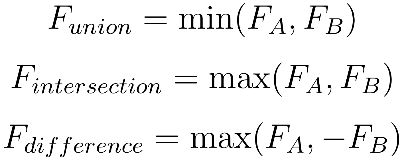
If you just wanted to make some basic 3D shapes, using the SDF form and then running MarchingCubes to mesh them, is not particularly efficient. The big advantage of SDFs is that you can easily combine shapes represented in SDF form by mathematically combining the SDF functions. A function that takes in one or more input SDFs, and generates an output SDF, is called an Operator.
The simplest compositions you can do with SDFs are the Boolean Operators Union, Intersection, and Difference. This is the complete opposite of meshes, where a mesh Boolean is incredibly difficult. With SDFs, Booleans are trivial to implement and always work (although you still have to mesh them!). The functions for the Boolean Operators are shown on the right. These are really just logical operations. Consider the Union, which is just the min() function. If you have two values, one less than 0 (inside) and one greater than 0 (outside), and you want to combine the two shapes, then you keep the smaller value.
The code below generates the three meshes shown in the figure on the right. Here the SDF primitives are a sphere and a box. From left to right we have Union, Difference, and Intersection. In this code we are using a function generateMeshF, you will find that function at the end of this post. It is just running MarchingCubes and writing the mesh to the given path.
ImplicitSphere3d sphere = new ImplicitSphere3d() {
    Origin = Vector3d.Zero, Radius = 1.0
};
ImplicitBox3d box = new ImplicitBox3d() {
    Box = new Box3d(new Frame3f(Vector3f.AxisX), 0.5*Vector3d.One)
};

generateMeshF(new ImplicitUnion3d() { A = sphere, B = box }, 128, "c:\\demo\\union.obj");
generateMeshF(new ImplicitDifference3d() { A = sphere, B = box }, 128, "c:\\demo\\difference.obj");
generateMeshF(new ImplicitIntersection3d() { A = sphere, B = box }, 128, "c:\\demo\\intersection.obj");
We are using Binary Operators in this sample code. g3Sharp also includes N-ary operators ImplicitNaryUnion3d and ImplicitNaryDifference3d. These just apply the same functions to sets of inputs.
Offset Surfaces

The Offset Surface operator is also trivial with SDFs. Remember, the surface is defined by distance == 0. If we wanted the surface to be shifted outwards by distance d, we could change the definition to distance == d. But we could also write this as (distance - d) == 0, and that's the entire code of the Offset Operator.
Just doing a single Offset of a Mesh SDF can be quite a powerful tool. The code below computes the inner and outer offset surfaces of the input mesh. If you wanted to, for example, Hollow a mesh for 3D printing, you can compute an inner offset at the desired wall thickness, flip the normals, and append it to the input mesh.
double offset = 0.2f;
DMesh3 mesh = TestUtil.LoadTestInputMesh("bunny_solid.obj");
MeshTransforms.Scale(mesh, 3.0 / mesh.CachedBounds.MaxDim);
BoundedImplicitFunction3d meshImplicit = meshToImplicitF(mesh, 64, offset);

generateMeshF(meshImplicit, 128, "c:\\demo\\mesh.obj");
generateMeshF(new ImplicitOffset3d() { A = meshImplicit, Offset = offset }, 128, "c:\\demo\\mesh_outset.obj");
generateMeshF(new ImplicitOffset3d() { A = meshImplicit, Offset = -offset }, 128, "c:\\demo\\mesh_inset.obj");
This code uses a function meshToImplicitF, which generates the Mesh SDF using the code from the Mesh SDF tutorial. I included this function at the end of the post.
Smooth Booleans
So far, we have only applied Operators to input Primitives. But we can also apply an Operator to another Operator. For example this code applies Offset to the Union of our sphere and box:
var union = new ImplicitUnion3d() { A = sphere, B = box };
generateMeshF(new ImplicitOffset3d() { A = union, Offset = offset }, 128, "c:\\demo\\union_offset.obj");
Now you could plug this Offset into another Operator. Very cool!
But, there's more we can do here. For example, what if we wanted this offset to have a smooth transition between the box and the sphere? The Min operator we use for the Boolean, has a discontinuity at the points where the two input functions are equal. What his means is, the output value abruptly "jumps" from one function to the other. Of course, this is what should happen on the surface, because a Boolean has a sharp transition from one shape to another. But it also happens in the "field" away from the surface. We don't see that field, but it affects the output of the Offset operation.

We can create a field that has a different shape by using a different equation for the Union operator. We will use the form on the right. If either A or B is zero, this function will still return the other value, so it still does a Min/Max operation. But if both values are non-zero, it combines them in a way that smoothly varies between A and B, instead of the sharp discontinuous jump.
Here's some sample code that generates our Offset example with this "SmoothUnion". The original box/sphere union looks the same, however in the Offset surface, the transition is smooth. This is because the
var smooth_union = new ImplicitSmoothDifference3d() { A = sphere, B = box };
generateMeshF(smooth_union, 128, "c:\\demo\\smooth_union.obj");
generateMeshF(new ImplicitOffset3d() { A = smooth_union, Offset = 0.2 }, 128, "c:\\demo\\smooth_union_offset.obj");
In this next section we will build on this SmoothUnion Operator, but first we need to cover one caveat. As I said above, if A and B are both non-zero, then this function produces a smooth combination of the input values. That's why we don't get the sharp transition. So, as you might expect, when we use d as the parameter to Offset, the offset distance in this smooth area cannot actually be d.
However, this smooth-composition happens everywhere in space, not just around the transition. As a result, the actual offset distance is affected everwhere as well. The figure on the right shows the original shape, then the discontinuous Offset, and finally the Smooth Offset. You can see that even on the areas that are "just sphere" and "just box", the Smooth Offset is a little bit bigger.
This is the price we pay for these "magic" smooth Operators. We gain continuity but we lose some of the nice metric properties. Mathematically, this happens because the the SmoothUnion operator produces a field that has properties similar to a Distance Field, but it's not actually a Distance Field. Specifically, it's not normalized, meaning if you computed the gradient and took it's magnitude, it would not be 1.
SmoothUnion is not just for shapes - it is called an R-Function, and R-functions implement Boolean logic using continuous functions, which has other applications. If this sounds interesting, here are a few starting points for further reading: [Shapiro88] [Shapiro07].
Blending Operator

By applying Offset to the SmoothUnion Operator, we can get a smooth transition in the offset surface. But what if we wanted that smooth transition between the input shapes, without the Offset? This is called a Blend Operator and is one of the biggest advantages of Implicit Modeling.
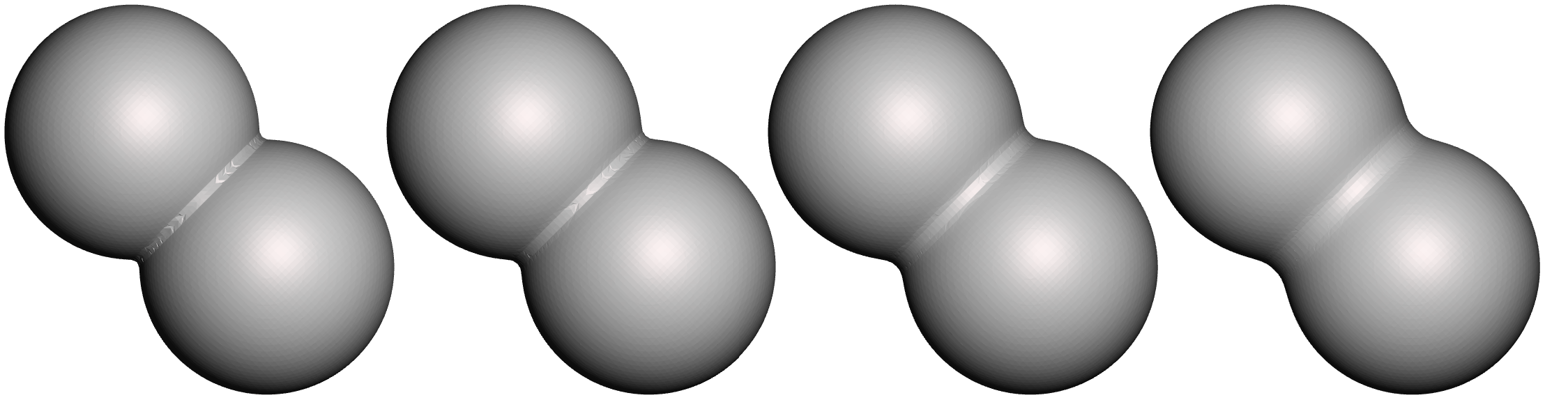
We will build Blend off of SmoothUnion. Basically, we want to vary the offset distance, so that if the point is close to both the input surfaces, we offset, and if it's only close to one of them, we don't. This variation needs to be smooth to produce a continuous blend. We use the equation above, based on [Pasko95], and implemented in ImplicitBlend3d. Here is an example, followed by the resulting blended spheres.
ImplicitSphere3d sphere1 = new ImplicitSphere3d() {
    Origin = Vector3d.Zero, Radius = 1.0
};
ImplicitSphere3d sphere2 = new ImplicitSphere3d() {
    Origin = 1.5 * Vector3d.AxisX, Radius = 1.0
};
generateMeshF(new ImplicitBlend3d() { A = sphere1, B = sphere2, Blend = 1.0 }, 128, "c:\\demo\\blend_1.obj");
generateMeshF(new ImplicitBlend3d() { A = sphere1, B = sphere2, Blend = 4.0 }, 128, "c:\\demo\\blend_4.obj");
generateMeshF(new ImplicitBlend3d() { A = sphere1, B = sphere2, Blend = 16.0 }, 128, "c:\\demo\\blend_16.obj");
generateMeshF(new ImplicitBlend3d() { A = sphere1, B = sphere2, Blend = 64.0 }, 128, "c:\\demo\\blend_64.obj");Mathematically, this blend is only C1 continous. As a result, although the surface is smooth, the variation in the normal is not. There are higher-order blending functions in [Pasko95], but they are computationally more intensive. Another aspect of this blend is that it has 3 parameters - w_blend, w_a, and w_b. Each of these affects the shape. In addition, the way they affect the shape depends on the scale of the distance values. In the example above, we used w_blend = 1,4,16,64. Each sphere had radius=1. If we use the same blending power with radius=2, we get different results:
It is possible to try to normalize w_blend based on, say, the bounding box of the input primitives. But, the per-shape weights w_a and w_b also come into play. If one shape is much smaller than the other, generally the larger one will "overwhelm" the smaller. You can use these weights to manipulate this effect. But changing these weights, also changes how much the blend surface deviates from the input surfaces in regions that are far from the places we would expect to see a blend.
Does this all sound complicated? It is! This is the trade-off with Implicit Modeling. We can have almost trivial, perfectly robust Booleans, Offsets, and Blending, but our tools to precisely control the surface are limited to abstract weights and functions. It is possible to, for example, vary the blending weights over space [Pasko05], based on some other function, to provide more control. Mathematically this is all pretty straightforward to implement, much easier than even a basic Laplacian mesh deformation. But, the fact that you can't just grab the surface and tweak it, tends to make Implicit Modeling difficult to use in some interactive design tools.
Mesh Blending
Lets apply our Blend Operator to some Mesh SDFs. The image on the right is produced by this sample code. As you can see, something has gone quite wrong...
DMesh3 mesh1 = TestUtil.LoadTestInputMesh("bunny_solid.obj");
MeshTransforms.Scale(mesh1, 3.0 / mesh1.CachedBounds.MaxDim);
DMesh3 mesh2 = new DMesh3(mesh1);
MeshTransforms.Rotate(mesh2, mesh2.CachedBounds.Center, Quaternionf.AxisAngleD(Vector3f.OneNormalized, 45.0f));

var meshImplicit1 = meshToImplicitF(mesh1, 64, 0);
var meshImplicit2 = meshToImplicitF(mesh2, 64, 0);
generateMeshF(new ImplicitBlend3d() { A = meshImplicit1, B = meshImplicit2, Blend = 0.0 }, 128, "c:\\demo\\blend_mesh_union.obj");
generateMeshF(new ImplicitBlend3d() { A = meshImplicit1, B = meshImplicit2, Blend = 10.0 }, 128, "c:\\demo\\blend_mesh_bad.obj");
What happened? Well, we didn't cover this in the Mesh SDF tutorial, but now we can explain a bit more about what MeshSignedDistanceGrid does. Remember, it samples the Distance Field of the input Mesh. But, samples it where? If we want to just mesh the SDF, we don't need the precise distance everywhere, we just need it near the surface. So, by default, this class only computes precise distances in a "Narrow Band" around the input mesh. Values in the rest of the sample grid are filled in using a "sweeping" technique that only sets the correct sign, not the correct distance. The ridges in the above image show the extent of the Narrow Band.
To get a better blend, we need to compute a full distance field, and the sampled field needs to extend far enough out to contain the blend region. This is much more expensive. The MeshSignedDistanceGrid class still only computes exact distances in a narrow band, but it will use a more expensive sweeping method which propagates more accurate distances. This is sufficient for blending. The meshToBlendImplicitF function (code at end of post) does this computation, and you can see the result of the sample code below on the right.
var meshFullImplicit1 = meshToBlendImplicitF(mesh1, 64);
var meshFullImplicit2 = meshToBlendImplicitF(mesh2, 64);
generateMeshF(new ImplicitBlend3d() { A = meshFullImplicit1, B = meshFullImplicit2, Blend = 1.0 }, 128, "c:\\demo\\blend_mesh_1.obj");
generateMeshF(new ImplicitBlend3d() { A = meshFullImplicit1, B = meshFullImplicit2, Blend = 10.0 }, 128, "c:\\demo\\blend_mesh_10.obj");
generateMeshF(new ImplicitBlend3d() { A = meshFullImplicit1, B = meshFullImplicit2, Blend = 50.0 }, 128, "c:\\demo\\blend_mesh_100.obj");
Lattice Demo
In the Mesh SDF post, I created a lattice by generating elements for each mesh edge. Now that we have these Primitives and Operators, we have some alternative ways to do this kind of thing. If we first Simplify our bunny mesh using this code:
DMesh3 mesh = TestUtil.LoadTestInputMesh("bunny_solid.obj");
MeshTransforms.Scale(mesh, 3.0 / mesh.CachedBounds.MaxDim);
MeshTransforms.Translate(mesh, -mesh.CachedBounds.Center);
Reducer r = new Reducer(mesh);
r.ReduceToTriangleCount(100);
And then use this following code to generate Line Primitives for each mesh edge and Union them:
double radius = 0.1;
List<BoundedImplicitFunction3d> Lines = new List<BoundedImplicitFunction3d>();
foreach (Index4i edge_info in mesh.Edges()) {
    var segment = new Segment3d(mesh.GetVertex(edge_info.a), mesh.GetVertex(edge_info.b));
    Lines.Add(new ImplicitLine3d() { Segment = segment, Radius = radius });
}
ImplicitNaryUnion3d unionN = new ImplicitNaryUnion3d() { Children = Lines };
generateMeshF(unionN, 128, "c:\\demo\\mesh_edges.obj");The result is an Analytic implicit 3D lattice. Now, say we wanted to strengthen the junctions.
We can just add in some spheres, and get the result on the right:
radius = 0.05;
List<BoundedImplicitFunction3d> Elements = new List<BoundedImplicitFunction3d>();
foreach (int eid in mesh.EdgeIndices()) {
    var segment = new Segment3d(mesh.GetEdgePoint(eid, 0), mesh.GetEdgePoint(eid, 1));
    Elements.Add(new ImplicitLine3d() { Segment = segment, Radius = radius });
}
foreach (Vector3d v in mesh.Vertices())
    Elements.Add(new ImplicitSphere3d() { Origin = v, Radius = 2 * radius });
generateMeshF(new ImplicitNaryUnion3d() { Children = Elements }, 256, "c:\\demo\\mesh_edges_and_vertices.obj");
Lightweighting Demo
Lightweighting in 3D printing is a process of taking a solid shape and reducing its weight, usually by adding hollow structures. There are sophisticated tools for this, like nTopology Element. But based on the tools we have so far, we can do some basic lightweighting in just a few lines of code. In this section we will hollow a mesh and fill the cavity with a grid pattern, entirely using Implicit modeling. The result is shown on the right (I cut away part of the shell to show the interior).
First we have a few parameters. These define the spacing of the lattice elements, and the wall thickness. This code is not particularly fast, so I would experiment using a low mesh resolution, and then turn it up for a nice result (and probably Reduce if you are planning to print it!).
double lattice_radius = 0.05;
double lattice_spacing = 0.4;
double shell_thickness = 0.05;
int mesh_resolution = 64;   // set to 256 for image quality
This is a bit of setup code that creates the Mesh SDF and finds the bounding boxes we will need
var shellMeshImplicit = meshToImplicitF(mesh, 128, shell_thickness);
double max_dim = mesh.CachedBounds.MaxDim;
AxisAlignedBox3d bounds = new AxisAlignedBox3d(mesh.CachedBounds.Center, max_dim / 2);
bounds.Expand(2 * lattice_spacing);
AxisAlignedBox2d element = new AxisAlignedBox2d(lattice_spacing);
AxisAlignedBox2d bounds_xy = new AxisAlignedBox2d(bounds.Min.xy, bounds.Max.xy);
AxisAlignedBox2d bounds_xz = new AxisAlignedBox2d(bounds.Min.xz, bounds.Max.xz);
AxisAlignedBox2d bounds_yz = new AxisAlignedBox2d(bounds.Min.yz, bounds.Max.yz);Now we make the 3D lattice. Note that we are making a full 3D tiling here, this has nothing to do with the input mesh shape. The image on the right shows what the lattice volume looks like. The code is just creating a bunch of line Primitives and then doing a giant Union.
List<BoundedImplicitFunction3d> Tiling = new List<BoundedImplicitFunction3d>();
foreach (Vector2d uv in TilingUtil.BoundedRegularTiling2(element, bounds_xy, 0)) {
    Segment3d seg = new Segment3d(new Vector3d(uv.x, uv.y, bounds.Min.z), new Vector3d(uv.x, uv.y, bounds.Max.z));
    Tiling.Add(new ImplicitLine3d() { Segment = seg, Radius = lattice_radius });
}
foreach (Vector2d uv in TilingUtil.BoundedRegularTiling2(element, bounds_xz, 0)) {
    Segment3d seg = new Segment3d(new Vector3d(uv.x, bounds.Min.y, uv.y), new Vector3d(uv.x, bounds.Max.y, uv.y));
    Tiling.Add(new ImplicitLine3d() { Segment = seg, Radius = lattice_radius });
}
foreach (Vector2d uv in TilingUtil.BoundedRegularTiling2(element, bounds_yz, 0)) {
    Segment3d seg = new Segment3d(new Vector3d(bounds.Min.x, uv.x, uv.y), new Vector3d(bounds.Max.x, uv.x, uv.y));
    Tiling.Add(new ImplicitLine3d() { Segment = seg, Radius = lattice_radius });
}
ImplicitNaryUnion3d lattice = new ImplicitNaryUnion3d() { Children = Tiling };
generateMeshF(lattice, 128, "c:\\demo\\lattice.obj");
These two lines Intersect the lattice with the Mesh SDF, clipping it against the input mesh. If you just wanted the inner lattice, you're done!
ImplicitIntersection3d lattice_clipped = new ImplicitIntersection3d() { A = lattice, B = shellMeshImplicit };
generateMeshF(lattice_clipped, mesh_resolution, "c:\\demo\\lattice_clipped.obj");
Now we make the shell, by subtracting an Offset of the Mesh SDF from the original Mesh SDF. Finally, we Union the shell and the clipped lattice, to get out result
var shell = new ImplicitDifference3d() {
    A = shellMeshImplicit,
    B = new ImplicitOffset3d() { A = shellMeshImplicit, Offset = -shell_thickness }
};
generateMeshF(new ImplicitUnion3d() { A = lattice_clipped, B = shell }, mesh_resolution, "c:\\demo\\lattice_result.obj");
That's it! If you wanted to, say, print this on a Formlabs printer, you might want to add some holes. This is easily done using additional operators. I'll leave it as an excerise to the reader =)
Ok, that's it. The remaining code is for the generateMeshF, meshToImplicitF, and meshToBlendImplicitF functions. Good luck!
// generateMeshF() meshes the input implicit function at
// the given cell resolution, and writes out the resulting mesh
Action<BoundedImplicitFunction3d, int, string> generateMeshF = (root, numcells, path) => {
    MarchingCubes c = new MarchingCubes();
    c.Implicit = root;
    c.RootMode = MarchingCubes.RootfindingModes.LerpSteps;      // cube-edge convergence method
    c.RootModeSteps = 5;                                        // number of iterations
    c.Bounds = root.Bounds();
    c.CubeSize = c.Bounds.MaxDim / numcells;
    c.Bounds.Expand(3 * c.CubeSize);                            // leave a buffer of cells
    c.Generate();
    MeshNormals.QuickCompute(c.Mesh);                           // generate normals
    StandardMeshWriter.WriteMesh(path, c.Mesh, WriteOptions.Defaults);   // write mesh
};

// meshToImplicitF() generates a narrow-band distance-field and
// returns it as an implicit surface, that can be combined with other implicits
Func<DMesh3, int, double, BoundedImplicitFunction3d> meshToImplicitF = (meshIn, numcells, max_offset) => {
    double meshCellsize = meshIn.CachedBounds.MaxDim / numcells;
    MeshSignedDistanceGrid levelSet = new MeshSignedDistanceGrid(meshIn, meshCellsize);
    levelSet.ExactBandWidth = (int)(max_offset / meshCellsize) + 1;
    levelSet.Compute();
    return new DenseGridTrilinearImplicit(levelSet.Grid, levelSet.GridOrigin, levelSet.CellSize);
};

// meshToBlendImplicitF() computes the full distance-field grid for the input
// mesh. The bounds are expanded quite a bit to allow for blending,
// probably more than necessary in most cases
Func<DMesh3, int, BoundedImplicitFunction3d> meshToBlendImplicitF = (meshIn, numcells) => {
    double meshCellsize = meshIn.CachedBounds.MaxDim / numcells;
    MeshSignedDistanceGrid levelSet = new MeshSignedDistanceGrid(meshIn, meshCellsize);
    levelSet.ExpandBounds = meshIn.CachedBounds.Diagonal * 0.25;        // need some values outside mesh
    levelSet.ComputeMode = MeshSignedDistanceGrid.ComputeModes.FullGrid;
    levelSet.Compute();
    return new DenseGridTrilinearImplicit(levelSet.Grid, levelSet.GridOrigin, levelSet.CellSize);
};